Friday, October 20, 2017

The retreat from religion is accelerating

Secularization in the Unites States

For more than a century religion in the the United States has defied gravity.  According to the Theory of Secularization, as societies become more modern, they become less religious.  Aspects of secularization include decreasing participation in organized religion, loss of religious belief, and declining respect for religious authority.  


Until recently the United States has been a nearly unique counterexample, so I would be a fool to join the line of researchers who have predicted the demise of religion in America.  Nevertheless, I predict that secularization in the U.S. will accelerate in the next 20 years.


Using data from the General Social Survey (GSS), I quantify changes since the 1970s in religious affiliation, belief, and attitudes toward religious authority, and present a demographic model that generates predictions.


Summary of results


Religious affiliation is changing quickly:


  • The fraction of people with no religious affiliation has increased from less than 10% in the 1990s to more than 20% now.  This increase will accelerate, overtaking Catholicism in the next few years, and probably replacing Protestantism as the largest religious affiliation within 20 years.
  • Protestantism has been in decline since the 1980s.  Its population share dropped below 50% in 2012, and will fall below 40% within 20 years.
  • Catholicism peaked in the 1980s and will decline slowly over the next 20 years, from 24% to 20%.
  • The share of other religions increased from 4% in the 1970s to 6% now, but will be essentially unchanged in the next 20 years.


Religious belief is in decline, as well as confidence in religious institutions:


  • The fraction of people who say they “know God really exists and I have no doubts about it” has decreased from 64% in the 1990s to 58% now, and will approach 50% in the next 20 years.
  • At the same time the share of atheists and agnostics, based on self-reports, has increased from 6% to 10%, and will reach 14% around 2030.
  • Confidence in the people running organized religions is dropping rapidly: the fraction who report a “great deal” of confidence has dropped from 36% in the 1970s to 19% now, while the fraction with “hardly any” has increased from 17% to 26%.  At 3-4 percentage points per decade, these are among the fastest changes we expect to see in this kind of data.
  • Interpretation of the Christian Bible has changed more slowly: the fraction of people who believe the Bible is “the actual word of God and is to be taken literally, word for word” has declined from 36% in the 1980s to 32% now, little more than 1 percentage point per decade.
  • At the same time the number of people who think the Bible is “an ancient book of fables, legends, history and moral precepts recorded by man” has nearly doubled, from 13% to 22%.  This skepticism will approach 30%, and probably overtake the literal interpretation, within 20 years.


Predictive demography


Let me explain where these predictions come from.  Since 1972 NORC at the University of Chicago has administered the General Social Survey (GSS), which surveys 1000-2000 adults in the U.S. per year.  The survey includes questions related to religious affiliation, attitudes, and beliefs.


Regarding religious affiliation, the GSS asks “What is your religious preference: is it Protestant, Catholic, Jewish, some other religion, or no religion?”  The following figure shows the results, with a 90% interval that quantifies uncertainty due to random sampling.


This figure provides an overview of trends in the population, but it is not easy to tell whether they are accelerating, and it does not provide a principled way to make predictions.  Nevertheless, demographic changes like this are highly predictable (at least compared to other kinds of social change).


Religious beliefs and attitudes are primarily determined by the environment people grow up in, including their family life and wider societal influences.  Although some people change religious affiliation later in life, most do not, so changes in the population are largely due to generational replacement.


We can get a better view of these changes if we group people by their year of birth, which captures information about the environment they grew up in, including the probability that they were raised in a religious tradition and their likely exposure to people of other religions.  The following figure shows the results:


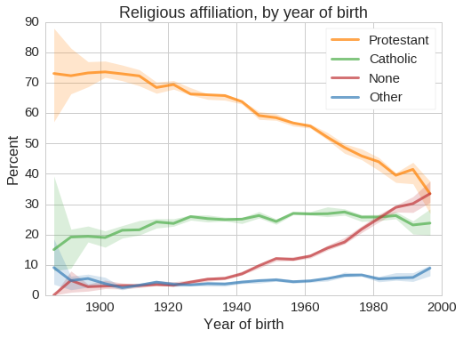
Among people born before 1940, a large majority are Protestant, only 20-25% are Catholic, and very few are Nones or Others.  These numbers have changed radically in the last few generations: among people born since 1980, there are more Nones than Catholics, and among the youngest adults, there may already be more Nones than Protestants.


However, this view of the data can be misleading.  Because these surveys were conducted between 1972 and the present, we observe different birth cohorts at different ages.  People born in 1900 were surveyed in their 70s and 80s, whereas people born in 1998 have only been observed at age 18.  If people tend to drift toward, or away from, religion as they age, we would have a biased view of the cohort effect.


Fortunately, with observations over more than 40 years, the design of the GSS makes it possible to estimate the effects of birth year and age simultaneously, using a regression model.  Then we can simulate the results of future surveys.  Here’s how:


  1. Each year, the GSS recruits a sample intended to represent the adult U.S. population, so the age range of the respondents is nearly the same every year.  We assume the set of ages will be the same for future surveys.
  2. Given the ages of hypothetical future respondents, we infer their years of birth.  For example, if we survey a 40-year-old in 2020, we know they were born in 1980.
  3. Given ages and years of birth, we use the regression model to predict the probability that each respondent will report being Protestant, Catholic, Other, or None.
  4. Then we use these probabilities to simulate survey results and predict the fraction of respondents in each group.


The following figure shows the results, with 90% intervals that represent uncertainty due to random sampling in the dataset and random variation in the simulations.


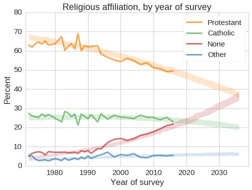
Over the next 20 years, the fraction of Protestants (including non-Catholic Christians) will decline quickly, falling below 40% around 2030.  The fraction of Catholics will decline more slowly, approaching 20%.  The fraction of other religions might increase slightly.


The fraction of “Nones” will increase quickly, overtaking Catholics in the next few years, and possibly becoming the largest religious group in the U.S. by 2036.


Are these predictions credible?


To see how reliable these predictions are, we can use past data to predict the present.  Supposing it’s 2006, and disregarding data from after 2006, the following figure shows the predictions we would make:


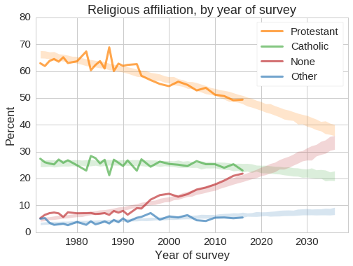
As it turns out, we would have been pretty much right, although we might have underpredicted the growth of the Nones.


Another reason to believe these predictions is that the events they predict have, in some sense, already happened.  The people who will be 40 years old in 2036 are 20 now, and we already have data about them.  The people who will be 20 in 2036 have already been born.


These predictions will be wrong if current teenagers are more religious than people in their 20s, or if current children are being raised in a more religious environment.  But if those things were happening, we would probably know.


In fact, these predictions are likely to be conservative:


  1. Survey results like these are notoriously subject to social desirability bias, which is the tendency of respondents to shade their answers in the direction they think is more socially acceptable.  To the degree that disaffiliation is stigmatized, we expect these reports to underestimate the number of Nones.
  2. The trend lines for Protestant and None have apparent points of inflection near 1990.  If we use only data since 1990 to build the model, we expect the Nones to reach 40% within 20 years.


Changes in religious belief


As affiliation with organized religion has declined, changes in religious belief have been relatively unchanged, a pattern that has been summarized as “believing without belonging”.  However there is evidence that believing will catch up with belonging over the next 20 years.


The GSS asks respondents, “Which statement comes closest to expressing what you believe about God?”
  1. I don't believe in God
  2. I don't know whether there is a God and I don't believe there is any way to find out
  3. I don't believe in a personal God, but I do believe in a Higher Power of some kind
  4. I find myself believing in God some of the time, but not at others
  5. While I have doubts, I feel that I do believe in God
  6. I know God really exists and I have no doubts about it


To make the number of categories more manageable, I classify responses 1 and 2 as “no belief”, responses 3, 4, and 5 as “belief”, and response 6 as “strong belief”.


The following figure shows how belief in God varies with year of birth.


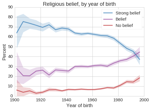
Among people born before 1940, more than 70% profess strong belief in God, but this confidence is in decline; among young adults fewer than 40% are so certain, and nearly 20% are either atheist or agnostic.


Again, we can use these results to model the effect of birth year and age, and use the model to generate predictions.  The following figure shows the results:


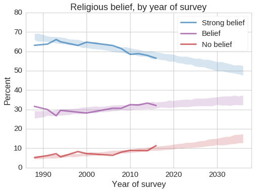
This question was added to the survey in 1988, and it has not been asked every year, so we have less data to work with.  Nevertheless, it is clear that strong belief in God is declining and being replaced by weaker forms of belief and non-belief.


Due to social desirability bias we can’t be sure what part of these trends is due to actual changes in belief, and how much might be the result of weakening stigmas against apostasy and atheism.  Regardless, these results indicate changes in what people say they believe.


Respect for religious authority


The GSS asks respondents, “As far as the people running [organized religion] are concerned, would you say you have a great deal of confidence, only some confidence, or hardly any confidence at all in them?”


The following figure shows how respect for religious authority varies with year of birth.


Among people born before 1940, 30 to 50% reported a “great deal” of confidence in the people running religious institutions.  Among young adults, this has dropped to 20%, and more than 25% now report “hardly any confidence at all”.


These changes have been going on for decades, and seem to be unrelated to specific events.  The following figures shows responses to the same question by year of survey.  The Catholic Church sexual abuse cases, which received widespread media attention starting in 1992, have no clear effect on the trends; if anything, confidence in religious institutions increased during the 1990s.


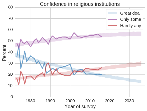
Predictions based on generational replacement suggest that these trends will continue.  Within 20 years, the fraction of people with hardly any confidence in religious institutions will approach 30%.


Interpretation of the Bible


The GSS asks, “Which one of these statements comes closest to describing your feelings about the Bible?”


  1. The Bible is the actual word of God and is to be taken literally, word for word.
  2. The Bible is the inspired word of God but not everything should be taken literally, word for word.
  3. The Bible is an ancient book of fables, legends, history and moral precepts recorded by man.


Responses to this question depend strongly on the respondents’ year of birth:


Among people born before 1940, more than 40% say they believe in a literal interpretation of the Christian Bible, and fewer than 15% consider it a collection of fables and legends.  Among young adults, these proportions have converged near 25%.


The number of people who believe that the Bible is the inspired word of God, but should not be interpreted literally, has been near 50% for several generations.  But this apparent equilibrium might mask two underlying trends: an increase due to transitions from literal to figurative interpretation, and a decrease due to transitions from “inspired” to “legends”.


The following figure shows responses to the same question over time, with predictions.

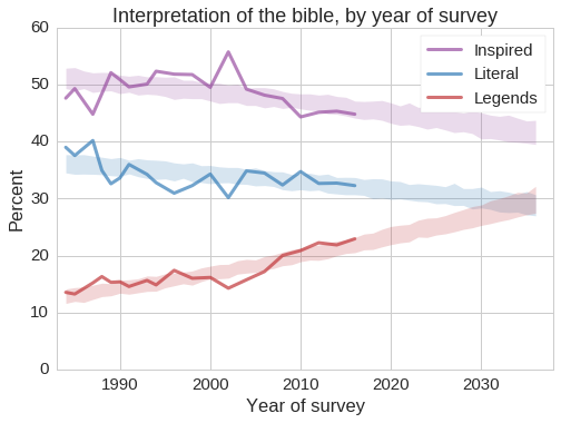
In the next 20 years, people who consider the Bible the literal or inspired word of God will be replaced by people who consider it a collection of ordinary documents, but this transition will be slow.


Again, these responses are susceptible to social desirability bias, so they may not reflect true beliefs accurately.  But they reflect changes in what people say they believe, which might cause a feedback effect: as more people express their non-belief, stigmas around atheism will decline, and these trends may accelerate.

Wednesday, June 14, 2017

Religion in the United States

Last night I had the pleasure of presenting a talk for the PyData Boston Meetup.  I presented a project I started earlier this summer, using data from the General Social Survey to measure and predict trends in religious affiliation and belief in the U.S.

The slides, which include the results so far and an overview of the methodology, are here:


And the code and data are all in this Jupyter notebook.  I'll post additional results and discussion over the next few weeks.

Thanks to Milos Miljkovic, organizer of the PyData Boston Meetup, for inviting me, and to O'Reilly Media for hosting the meeting.

Thursday, June 1, 2017

Spring 2017 Data Science reports

In my Data Science class this semester, students worked on a series of reports where they explore a freely-available dataset, use data to answer questions, and present their findings.  After each batch of reports, I will publish the abstracts here; you can follow the links below to see what they found.


How Do You Predict Who Will Vote?

Sean Carter

One topic that enters popular discussion every four years is "who votes?" Every presidential election we see many discussions on which groups are more likely to vote, and which important voter groups each candidate needs to capture. One theme that is often part of this discussion is whether or not a candidate's biggest support is among groups likely to turn out. This analysis of the General Social Survey uses a number of different demographic variables to try and answer that question. Report


Designing the Optimal Employee Experience... For Employers

Joey Maalouf

Using a dataset published by Medium on Kaggle, I explored the relationship between an employee's working conditions and the likelihood that they will quit their job. There were some expected trends, like lower salary leading to a higher attrition rate, but also some surprising ones, like having an accident at work leading to a lower likelihood of quitting! This observed information can be used by employers to determine the quitting probability of a specific individual, or to calculate the attrition rate of a larger group, like a department, and adjust their conditions accordingly.
Report


Does being married have an effect on your political views?

Apurva Raman and William Lu

Politics has often been a polarizing subject amongst Americans, and in today's increasingly partisan political environment, that has not changed. Using data from the General Social Survey (GSS), an annual study designed and conducted by the National Opinion Research Center (NORC) at the University of Chicago, we identify variables that are correlated with a person's political views. We find that while marital status has a statistically significant apparent effect on political views, that apparent effect is drastically reduced when including confounding variables, particularly religion. Report


Should you Follow the Food Groups for Dietary Advice?

Kaitlyn Keil and Kevin Zhang

In the 1990s, the USDA put out the image of a Food Guide Pyramid to help direct dietary choices. It grouped foods into six categories: grains, proteins (meats, fish, eggs, etc), vegetables, fruits, dairy, and fats and oils. Since then, the pyramid has been revamped in 2005, and then pushed towards a plate with five categories (oils were dropped) in the 2010s. The general population has learned of these basic food groups since grade school, and over time either fully adopts them into their lifestyles, or abandons them to pursue their own balanced diet. In light of the controversy surrounding the Food Pyramid, we decided to ask whether the food categories found in the Food Pyramid truly represent the correct groupings for food, and if not, just how far off are they? Using K-Means clustering on an extensive food databank, we created 6 groupings of food based on their macronutrient composition, which was the primary criteria the original Food Pyramid used in its categorization. We found that the K-Means groups only overlapped with existing food groups from the Food Pyramid 50% of the time, potentially suggesting that the idea of the basic food groups could be outdated. Report


Are Terms of Home Mortgage Less Favorable Now Compared to Pre Mortgage Crisis?

Sungwoo Park

It is well known fact that excessive amount of default from subprime mortgages, which are mortgages normally issued to a borrower of low credit, was a leading cause of subprime mortgage crisis that led to a global financial meltdown in 2007. Because of this nightmarish experience, it seems plausible to assume that current home mortgages are much harder to get and much more conservative (in terms of risks the lender is taking, shown mainly as an interest rate) than pre-2007 mortgages. Using a dataset containing all home mortgages purchased or guaranteed from The Federal Home Loan Mortgage Corporation, more commonly known as Freddie Mac, I investigate whether there is any noticeable difference between the interest rates before and after subprime mortgage crisis.
Report


Finding NBA Players with Similar Styles

Willem Thorbecke and David Papp

Players in the NBA are often compared to others, both active and retired, based on similar play styles. For example, it is common to hear statements such as “Russell Westbrook is the new Derrick Rose”. The purpose of our project is to apply machine learning in the form of clustering to see which players are actually similar based on 22 variables. We successfully generated clusters of players that are very similar quantitatively. It is up to the reader to decide whether this is qualitatively true. Report


Food Trinities and Recipe Completion

Matt Ruehle

We can tell where a food is from - at least, culturally - from just a few bites. There are palettes of ingredients and spices which are strongly associated with each other - giving cajun cooking its kick, and french cuisine its "je ne sais quoi." But, what exactly these palettes and pairings are varies - ask ten different chefs, and you'll get six different answers. We look for a statistical way to identify "trinities" like "onion, carrot, celery" or "garlic, sesame oil, soy sauce," in the process both finding several associations not typically reflected in culinary literature and creating a tool which extends recipes based on their already-known ingredients, in a manner akin to a food version of a cell phone's autocomplete. Report


All the News in 2010 and 2012

Radmer van der Heyde

I examined the Pew News Coverage Index dataset from the years 2010 and 2012 to see how the different topics and stories were covered across media sectors and sources. The combined dataset had over 70,000 stories from all media sectors: print, online, cable tv, network tv, and broadcast radio. From the data, topics have less variance in word count and duration than sources. Report


Wednesday, April 26, 2017

Python as a way of thinking

This article contains supporting material for this blog post at Scientific American.  The thesis of the post is that modern programming languages (like Python) are qualitatively different from the first generation (like FORTRAN and C), in ways that make them effective tools for teaching, learning, exploring, and thinking.

I presented a longer version of this argument in a talk I presented at Olin College last fall.  The slides are here:


Here are Jupyter notebooks with the code examples I mentioned in the talk:

Here's my presentation at SciPy 2015, where I talked more about Python as a way of teaching and learning DSP:


Finally, here's the notebook "Using Counters", which uses Python's Counter object to implement a PMF (probability mass function) and perform Bayesian updates.

In [13]:
from __future__ import print_function, division

from collections import Counter
import numpy as np
A counter is a map from values to their frequencies. If you initialize a counter with a string, you get a map from each letter to the number of times it appears. If two words are anagrams, they yield equal Counters, so you can use Counters to test anagrams in linear time.
In [3]:
def is_anagram(word1, word2):
    """Checks whether the words are anagrams.

    word1: string
    word2: string

    returns: boolean
    """
    return Counter(word1) == Counter(word2)
In [4]:
is_anagram('tachymetric', 'mccarthyite')
Out[4]:
True
In [5]:
is_anagram('banana', 'peach')
Out[5]:
False
Multisets
A Counter is a natural representation of a multiset, which is a set where the elements can appear more than once. You can extend Counter with set operations like is_subset:
In [6]:
class Multiset(Counter):
    """A multiset is a set where elements can appear more than once."""

    def is_subset(self, other):
        """Checks whether self is a subset of other.

        other: Multiset

        returns: boolean
        """
        for char, count in self.items():
            if other[char] < count:
                return False
        return True
    
    # map the <= operator to is_subset
    __le__ = is_subset
You could use is_subset in a game like Scrabble to see if a given set of tiles can be used to spell a given word.
In [7]:
def can_spell(word, tiles):
    """Checks whether a set of tiles can spell a word.

    word: string
    tiles: string

    returns: boolean
    """
    return Multiset(word) <= Multiset(tiles)
In [8]:
can_spell('SYZYGY', 'AGSYYYZ')
Out[8]:
True

Probability Mass Functions

You can also extend Counter to represent a probability mass function (PMF).
normalize computes the total of the frequencies and divides through, yielding probabilities that add to 1.
__add__ enumerates all pairs of value and returns a new Pmf that represents the distribution of the sum.
__hash__ and __id__ make Pmfs hashable; this is not the best way to do it, because they are mutable. So this implementation comes with a warning that if you use a Pmf as a key, you should not modify it. A better alternative would be to define a frozen Pmf.
render returns the values and probabilities in a form ready for plotting
In [9]:
class Pmf(Counter):
    """A Counter with probabilities."""

    def normalize(self):
        """Normalizes the PMF so the probabilities add to 1."""
        total = float(sum(self.values()))
        for key in self:
            self[key] /= total

    def __add__(self, other):
        """Adds two distributions.

        The result is the distribution of sums of values from the
        two distributions.

        other: Pmf

        returns: new Pmf
        """
        pmf = Pmf()
        for key1, prob1 in self.items():
            for key2, prob2 in other.items():
                pmf[key1 + key2] += prob1 * prob2
        return pmf

    def __hash__(self):
        """Returns an integer hash value."""
        return id(self)
    
    def __eq__(self, other):
        return self is other

    def render(self):
        """Returns values and their probabilities, suitable for plotting."""
        return zip(*sorted(self.items()))
As an example, we can make a Pmf object that represents a 6-sided die.
In [10]:
d6 = Pmf([1,2,3,4,5,6])
d6.normalize()
d6.name = 'one die'
print(d6)
Pmf({1: 0.16666666666666666, 2: 0.16666666666666666, 3: 0.16666666666666666, 4: 0.16666666666666666, 5: 0.16666666666666666, 6: 0.16666666666666666})
Using the add operator, we can compute the distribution for the sum of two dice.
In [11]:
d6_twice = d6 + d6
d6_twice.name = 'two dice'

for key, prob in d6_twice.items():
    print(key, prob)
2 0.0277777777778
3 0.0555555555556
4 0.0833333333333
5 0.111111111111
6 0.138888888889
7 0.166666666667
8 0.138888888889
9 0.111111111111
10 0.0833333333333
11 0.0555555555556
12 0.0277777777778
Using numpy.sum, we can compute the distribution for the sum of three dice.
In [14]:
# if we use the built-in sum we have to provide a Pmf additive identity value
# pmf_ident = Pmf([0])
# d6_thrice = sum([d6]*3, pmf_ident)

# with np.sum, we don't need an identity
d6_thrice = np.sum([d6, d6, d6])
d6_thrice.name = 'three dice'
And then plot the results (using Pmf.render)
In [19]:
import matplotlib.pyplot as plt
%matplotlib inline
In [20]:
for die in [d6, d6_twice, d6_thrice]:
    xs, ys = die.render()
    plt.plot(xs, ys, label=die.name, linewidth=3, alpha=0.5)
    
plt.xlabel('Total')
plt.ylabel('Probability')
plt.legend()
plt.show()

Bayesian statistics

A Suite is a Pmf that represents a set of hypotheses and their probabilities; it provides bayesian_update, which updates the probability of the hypotheses based on new data.
Suite is an abstract parent class; child classes should provide a likelihood method that evaluates the likelihood of the data under a given hypothesis. update_bayesian loops through the hypothesis, evaluates the likelihood of the data under each hypothesis, and updates the probabilities accordingly. Then it re-normalizes the PMF.
In [21]:
class Suite(Pmf):
    """Map from hypothesis to probability."""

    def bayesian_update(self, data):
        """Performs a Bayesian update.
        
        Note: called bayesian_update to avoid overriding dict.update

        data: result of a die roll
        """
        for hypo in self:
            like = self.likelihood(data, hypo)
            self[hypo] *= like

        self.normalize()
As an example, I'll use Suite to solve the "Dice Problem," from Chapter 3 of Think Bayes.
"Suppose I have a box of dice that contains a 4-sided die, a 6-sided die, an 8-sided die, a 12-sided die, and a 20-sided die. If you have ever played Dungeons & Dragons, you know what I am talking about. Suppose I select a die from the box at random, roll it, and get a 6. What is the probability that I rolled each die?"
I'll start by making a list of Pmfs to represent the dice:
In [31]:
def make_die(num_sides):
    die = Pmf(range(1, num_sides+1))
    die.name = 'd' + str(num_sides)
    die.normalize()
    return die

dice = [make_die(x) for x in [4, 6, 8, 12, 20]]
for die in dice:
    print(die)
Pmf({1: 0.25, 2: 0.25, 3: 0.25, 4: 0.25})
Pmf({1: 0.16666666666666666, 2: 0.16666666666666666, 3: 0.16666666666666666, 4: 0.16666666666666666, 5: 0.16666666666666666, 6: 0.16666666666666666})
Pmf({1: 0.125, 2: 0.125, 3: 0.125, 4: 0.125, 5: 0.125, 6: 0.125, 7: 0.125, 8: 0.125})
Pmf({1: 0.08333333333333333, 2: 0.08333333333333333, 3: 0.08333333333333333, 4: 0.08333333333333333, 5: 0.08333333333333333, 6: 0.08333333333333333, 7: 0.08333333333333333, 8: 0.08333333333333333, 9: 0.08333333333333333, 10: 0.08333333333333333, 11: 0.08333333333333333, 12: 0.08333333333333333})
Pmf({1: 0.05, 2: 0.05, 3: 0.05, 4: 0.05, 5: 0.05, 6: 0.05, 7: 0.05, 8: 0.05, 9: 0.05, 10: 0.05, 11: 0.05, 12: 0.05, 13: 0.05, 14: 0.05, 15: 0.05, 16: 0.05, 17: 0.05, 18: 0.05, 19: 0.05, 20: 0.05})
Next I'll define DiceSuite, which inherits bayesian_update from Suite and provides likelihood.
data is the observed die roll, 6 in the example.
hypo is the hypothetical die I might have rolled; to get the likelihood of the data, I select, from the given die, the probability of the given value.
In [26]:
class DiceSuite(Suite):
    
    def likelihood(self, data, hypo):
        """Computes the likelihood of the data under the hypothesis.

        data: result of a die roll
        hypo: Pmf object representing a die
        """
        return hypo[data]
Finally, I use the list of dice to instantiate a Suite that maps from each die to its prior probability. By default, all dice have the same prior.
Then I update the distribution with the given value and print the results:
In [33]:
dice_suite = DiceSuite(dice)

dice_suite.bayesian_update(6)

for die in sorted(dice_suite):
    print(len(die), dice_suite[die])
4 0.0
6 0.392156862745
8 0.294117647059
12 0.196078431373
20 0.117647058824
As expected, the 4-sided die has been eliminated; it now has 0 probability. The 6-sided die is the most likely, but the 8-sided die is still quite possible.
Now suppose I roll the die again and get an 8. We can update the Suite again with the new data
In [30]:
dice_suite.bayesian_update(8)

for die, prob in sorted(dice_suite.items()):
    print(die.name, prob)
d4 0.0
d6 0.0
d8 0.623268698061
d12 0.277008310249
d20 0.0997229916898
Now the 6-sided die has been eliminated, the 8-sided die is most likely, and there is less than a 10% chance that I am rolling a 20-sided die.
These examples demonstrate the versatility of the Counter class, one of Python's underused data structures.
In [ ]: